Presidential speech across eras

A worked gallery: comparing the vocabulary of U.S. presidential speeches across 25-year eras with keyness, rank-turbulence divergence, and the allotaxonograph.

The data are compact frequency tables under examples/data/, built from the public-domain Miller Center presidential speech corpus (lemmatised, lowercased, punctuation stripped) bundled with chronowords, loaded with keyflux.load_counts. A light filter drops clitic fragments and transcription markers; genuine function words stay in (they populate the lockword diagonal).

The full, executed notebook — with every figure inline — is at examples/presidential_speeches.ipynb.

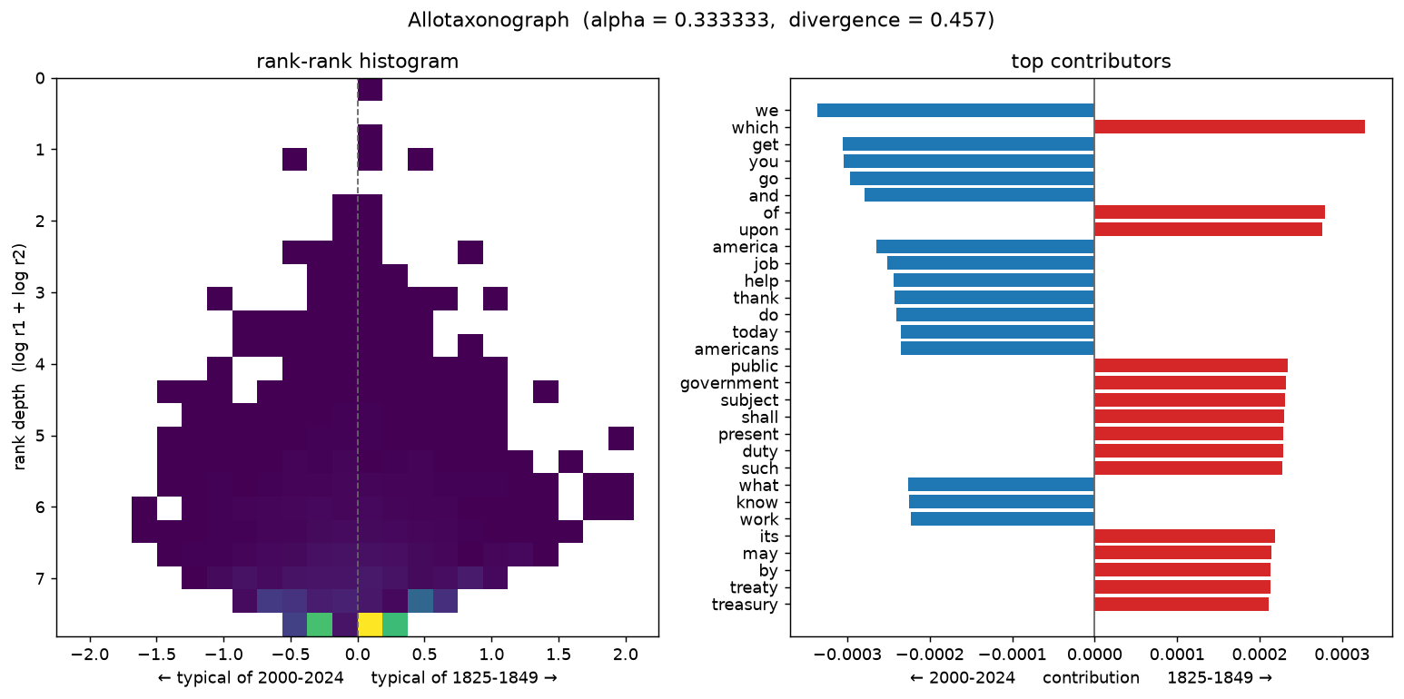
1. The nineteenth century vs. the twenty-first

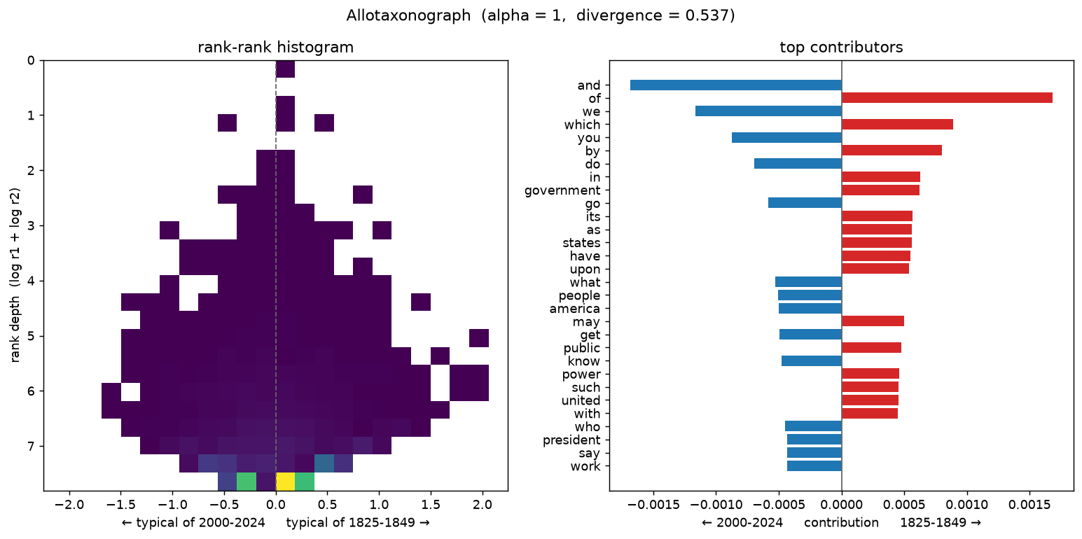
The starkest shift: formal 19th-century governmental prose against modern televised address. Positive keywords for 2000–2024: job, help, today, tonight, worker, terrorist, afghanistan, billion. For 1825–1849: appropriation, intercourse, specie, heretofore, receipt, treasury. The contribution panel reads first-person modern (we, get, help, thank, americans) against formal 19th-century register (which, upon, shall, duty, treaty).

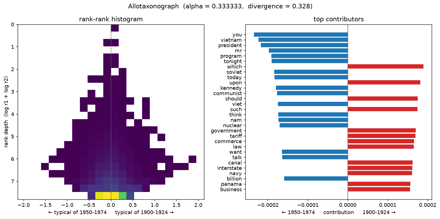
2. The Progressive era vs. the Cold War

1950–1974 keywords: vietnam, soviet, kennedy, communist, nuclear, nixon. 1900–1924 keywords: railway, isthmus, philippine, hague, reclamation, banking — the vocabulary of the Panama Canal, imperial expansion, and early regulation.

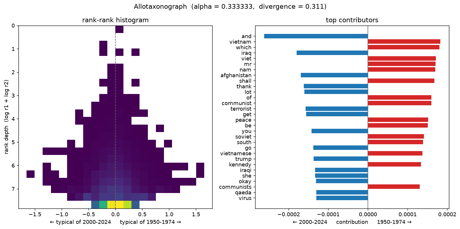
3. The Cold War vs. the modern era

A more recent, subtler shift. 2000–2024: afghanistan, iraqi, qaeda, virus, ukraine, biden. 1950–1974: viet, nam, communists, khrushchev, watergate, laos, mcnamara.

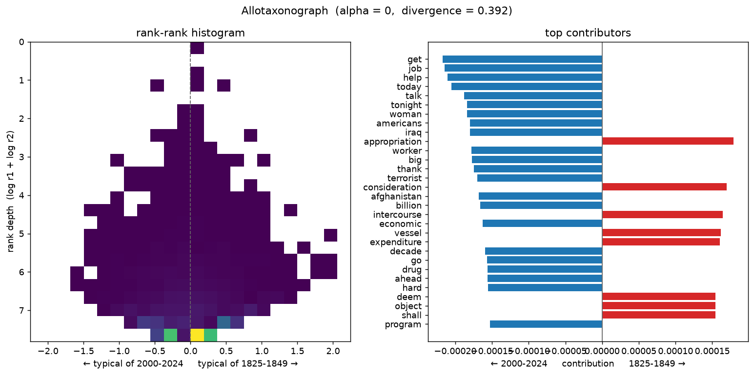
How alpha reframes the map

alpha tunes what the divergence emphasises — small alpha surfaces churn among rare, low-rank words; large alpha surfaces shifts among common, high-rank words. The 19thC↔21stC pair at three settings (divergence rises from 0.39 to 0.54):

alpha = 0 (logarithmic limit — rare, low-rank churn)

alpha = 1/3 (the text default)

alpha = 1 (emphasises common, high-rank words)

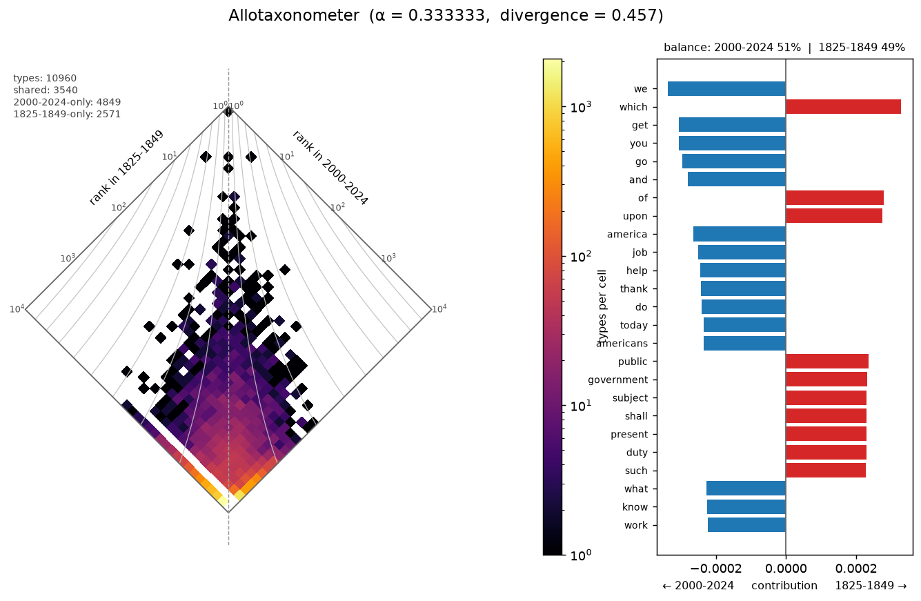
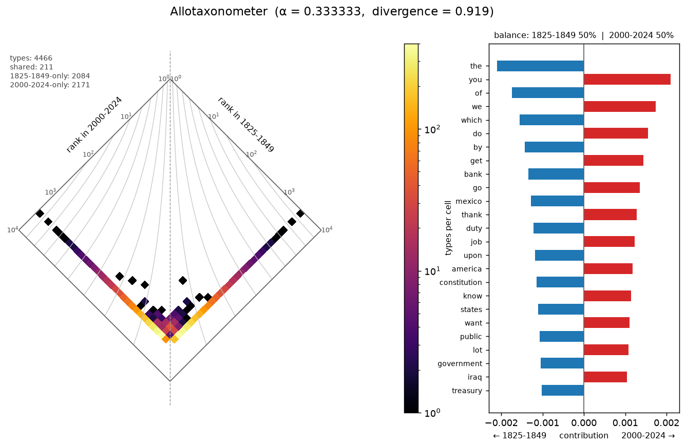
The diamond allotaxonograph

The same comparison in the canonical Dodds (2020) diamond (allotaxonometer): a rotated-square rank-rank histogram with iso-divergence contours and a wordshift list. Shared function words sit on the vertical centre near the top; era-specific and exclusive words fan out to the lower edges.

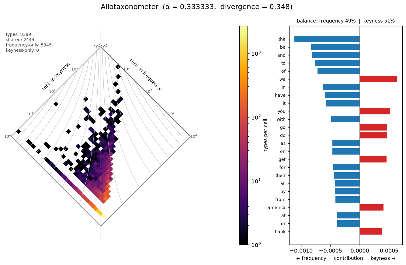
Frequent words vs. keywords — two rankings of one corpus

allotaxonometer compares any two rankings, not just two corpora. Here the 2000–2024 corpus is ranked two ways — by raw frequency and by keyness (log-likelihood vs the 1825–1849 reference, via RankedList.from_scores) — and diamonded against itself. Read the two edges as the two rankings: the right edge is a word's rank in frequency, the left edge its rank in keyness. A word leaning right (blue) is frequent but not distinctive — the function words the, be, and, of; a word leaning left (red) is distinctive but not among the most frequent — we, you, america, thank. The bright edge is the ~5,900 words that are frequent but aren't positive keywords, so they have no keyness rank. Same vocabulary, reordered.

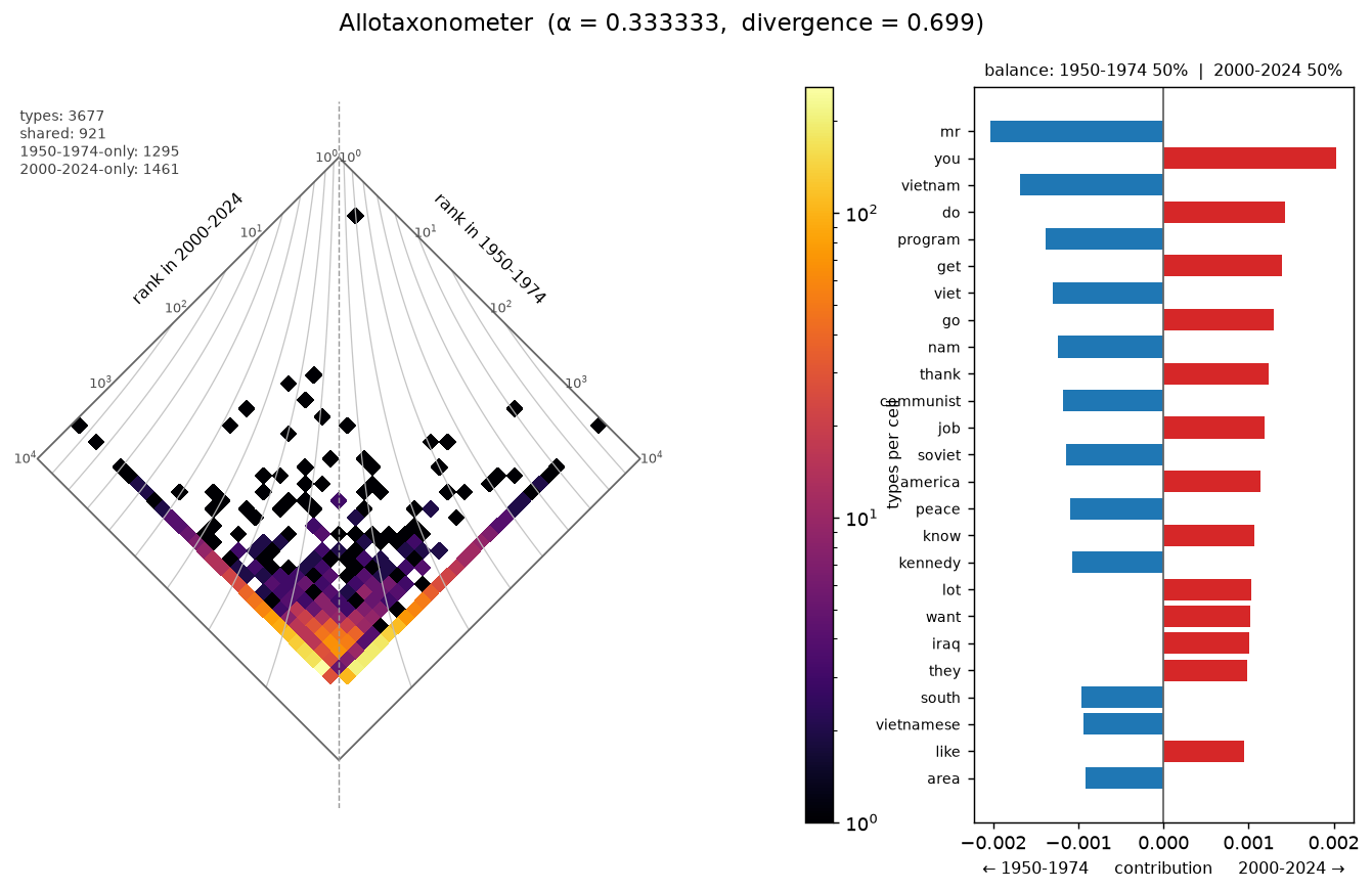
Keyness vs. keyness across eras

Keyness always needs a reference, so to compare eras on equal footing we give each era the same reference — the rest of the presidential corpus (all other eras combined) — and rank its over-represented words by keyness (RankedList.from_scores). Each ranking is then an era's distinctive vocabulary versus the tradition. Diamonding two eras' keyness rankings shows which words are distinctive of both (near the top centre) and which are distinctive of only one (fanning to its side); the divergence measures how differently the two eras stand out.

Cold War (1950–1974) vs. modern (2000–2024). Distinctive of 1950–1974: vietnam, program, communist, soviet, peace, kennedy. Distinctive of 2000–2024: you, do, get, thank, job, america, iraq. Their distinctive vocabularies barely overlap — divergence ≈ 0.70.

Nineteenth century (1825–1849) vs. twenty-first (2000–2024).

The script

examples/presidential_speeches.py

# %% [markdown]
# # Allotaxonographs of U.S. presidential speech across eras
#
# This example compares the vocabulary of U.S. presidential speeches across
# 25-year eras with **keyflux** — keyness (keywords + lockwords), rank-turbulence
# divergence (RTD), and the allotaxonograph.
#
# The data are compact frequency tables under `examples/data/`, built from the
# public-domain [Miller Center](https://data.millercenter.org/) presidential
# speech corpus (lemmatised, lowercased, punctuation stripped) bundled with
# [chronowords](https://github.com/crow-intelligence/chronowords). Each table is
# `type<TAB>count`, trimmed to count ≥ 2, and is loaded with `keyflux.load_counts`.

# %%
from collections import Counter
from pathlib import Path

from keyflux import (
    Keyness,
    RankedList,
    allotaxonograph,
    allotaxonometer,
    load_counts,
    rtd,
)

try:
    HERE = Path(__file__).resolve().parent
except NameError:  # running as a notebook — no __file__
    HERE = Path("examples") if Path("examples/data").exists() else Path(".")
DATA = HERE / "data"
GALLERY = HERE / "gallery"
GALLERY.mkdir(exist_ok=True)

# Lemmatisation and transcription leave clitic fragments (ve, ll, re) and stage
# markers ([applause], speaker labels). They are real tokens but pure noise, so
# we drop them from the counts up front — this keeps genuine function words (the,
# of, be, which), which legitimately populate the lockword diagonal.
_NOISE = {
    "ve", "ll", "re", "s", "d", "m", "t", "s1", "s2", "p1", "p2",
    "applause", "laughter", "crosstalk", "inaudible", "span", "class",
    "nbsp", "amp", "quot", "don", "didn", "doesn", "isn", "aren", "wasn",
    "won", "wouldn", "couldn", "shouldn", "hasn", "haven", "uh", "um",
}


def clean(counter):
    """Drop single-character tokens and known clitic/transcript noise."""
    return Counter({t: c for t, c in counter.items() if len(t) > 1 and t not in _NOISE})


PERIODS = ["1825-1849", "1900-1924", "1950-1974", "2000-2024"]
counts = {p: clean(load_counts(DATA / f"speeches_{p}.tsv")) for p in PERIODS}
for p in PERIODS:
    print(f"{p}: {sum(counts[p].values()):>8,} tokens, {len(counts[p]):>6,} types")


def content_words(rows, n=12):
    """Top keyword surface forms for the printed lists."""
    return [row.type for row in rows[:n]]


def show(fig):
    """Embed a Figure as a PNG output when run in a notebook; no-op in a script."""
    try:
        from io import BytesIO

        from IPython.display import Image, display
    except ImportError:
        return
    buf = BytesIO()
    fig.savefig(buf, format="png", dpi=110, bbox_inches="tight")
    display(Image(data=buf.getvalue()))


# %% [markdown]
# ## The comparison helper
#
# For a focus era vs. a reference era it prints the positive keywords (typical of
# the focus era), the negative keywords (typical of the reference era), and a few
# lockwords (stable across both), then renders the allotaxonograph.


# %%
def compare(focus_period, reference_period, *, alpha=1 / 3, save_as=None):
    """Keyness + RTD + allotaxonograph for two eras; returns the Figure."""
    focus, reference = counts[focus_period], counts[reference_period]
    k = Keyness(
        focus, reference,
        min_focus_freq=10, min_reference_freq=10,
        reference_id=reference_period,
    )
    kw = k.keywords()
    print(f"\n=== {focus_period}  vs  {reference_period} ===")
    print(f"typical of {focus_period}:   {content_words(kw.positive())}")
    print(f"typical of {reference_period}:   {content_words(kw.negative())}")
    print(f"lockwords (stable):   {content_words(k.lockwords(min_freq_both=50))}")

    r_focus = RankedList.from_counts(focus, label=focus_period)
    r_reference = RankedList.from_counts(reference, label=reference_period)
    result = rtd(r_focus, r_reference, alpha=alpha)
    print(f"rank-turbulence divergence (alpha={alpha:.3g}): {result.divergence:.4f}")

    fig = allotaxonograph(
        r_focus, r_reference, alpha=alpha,
        labels=(focus_period, reference_period),
    )
    if save_as:
        fig.savefig(GALLERY / save_as, dpi=130, bbox_inches="tight")
        print(f"saved gallery/{save_as}")
    return fig


# %% [markdown]
# ## 1. The nineteenth century vs. the twenty-first
#
# The most dramatic shift: formal 19th-century governmental prose
# (*appropriation, intercourse, specie*) against modern televised address
# (*job, help, tonight*). Function words fill the lockword diagonal.

# %%
fig1 = compare("2000-2024", "1825-1849", save_as="era_2000-2024_vs_1825-1849.png")
show(fig1)

# %% [markdown]
# ## 2. Progressive era vs. the Cold War

# %%
fig2 = compare("1950-1974", "1900-1924", save_as="era_1950-1974_vs_1900-1924.png")
show(fig2)

# %% [markdown]
# ## 3. The Cold War vs. the modern era — a subtler shift

# %%
fig3 = compare("2000-2024", "1950-1974", save_as="era_2000-2024_vs_1950-1974.png")
show(fig3)

# %% [markdown]
# ## How alpha reframes the map
#
# `alpha` tunes what the divergence emphasises. Small `alpha` surfaces churn
# among rare, low-rank words; large `alpha` surfaces shifts among the common,
# high-rank words. Here is the 19thC↔21stC pair at three settings.

# %%
for a, tag in [(0.0, "0"), (1 / 3, "0.33"), (1.0, "1")]:
    fig = compare("2000-2024", "1825-1849", alpha=a,
                  save_as=f"alpha_sweep_{tag}.png")
    show(fig)

# %% [markdown]
# ## The diamond allotaxonograph (`allotaxonometer`)
#
# The same comparisons in the canonical Dodds (2020) diamond: a rotated-square
# rank-rank histogram with iso-divergence contours and a wordshift list. Shared
# function words sit on the vertical centre near the top; era-specific and
# exclusive words fan out to the edges.


# %%
def diamond(focus_period, reference_period, *, alpha=1 / 3, save_as=None):
    """Render the diamond allotaxonograph for two eras; returns the Figure."""
    r_focus = RankedList.from_counts(counts[focus_period], label=focus_period)
    r_reference = RankedList.from_counts(
        counts[reference_period], label=reference_period
    )
    fig = allotaxonometer(r_focus, r_reference, alpha=alpha)
    if save_as:
        fig.savefig(GALLERY / save_as, dpi=130, bbox_inches="tight")
        print(f"saved gallery/{save_as}")
    return fig


# %%
show(diamond("2000-2024", "1825-1849", save_as="diamond_2000-2024_vs_1825-1849.png"))

# %%
show(diamond("2000-2024", "1950-1974", save_as="diamond_2000-2024_vs_1950-1974.png"))

# %% [markdown]
# ## Frequent words vs. keywords — two rankings of one corpus
#
# `allotaxonometer` compares *any* two rankings. Here we rank the 2000–2024
# corpus two ways — by raw frequency and by keyness (log-likelihood vs the
# 1825–1849 reference, via `RankedList.from_scores`) — and diamond them against
# each other. Function words top the frequency ranking but vanish from the
# keyness ranking; content words leap up. It's the same vocabulary, reordered.

# %%
freq_rank = RankedList.from_counts(counts["2000-2024"], label="frequency")
_k = Keyness(counts["2000-2024"], counts["1825-1849"],
             min_focus_freq=10, min_reference_freq=10)
key_scores = {r.type: r.statistic for r in _k.table() if r.direction == "positive"}
key_rank = RankedList.from_scores(key_scores, label="keyness")
fig_fk = allotaxonometer(freq_rank, key_rank, alpha=1 / 3)
fig_fk.savefig(
    GALLERY / "diamond_frequency_vs_keyness.png", dpi=130, bbox_inches="tight"
)
print("saved gallery/diamond_frequency_vs_keyness.png")
show(fig_fk)

# %% [markdown]
# ## Keyness vs. keyness — which words are distinctive of each era
#
# Keyness always needs a reference. To compare *eras* on equal footing we give
# each era the **same** reference: the rest of the presidential corpus (all other
# eras combined). For each era we rank its over-represented words by keyness
# (log-likelihood, `RankedList.from_scores`) — its "distinctive vocabulary" — and
# diamond two eras' keyness rankings against each other. Words distinctive of
# *both* compared eras (versus the tradition) sit near the top centre; words
# distinctive of only one era fan out to its side; the divergence measures how
# differently the two eras stand out.


# %%
def era_keyness_ranking(period, *, min_freq=10):
    """Rank a period's over-represented words by keyness vs the rest of the corpus."""
    rest = Counter()
    for other, c in counts.items():
        if other != period:
            rest.update(c)
    k = Keyness(
        counts[period], rest, min_focus_freq=min_freq, min_reference_freq=min_freq
    )
    scores = {r.type: r.statistic for r in k.table() if r.direction == "positive"}
    return RankedList.from_scores(scores, label=period)


def keyness_diamond(period_a, period_b, *, alpha=1 / 3, save_as=None):
    """Diamond two eras' keyness rankings (each vs the rest of the corpus)."""
    fig = allotaxonometer(
        era_keyness_ranking(period_a), era_keyness_ranking(period_b), alpha=alpha
    )
    if save_as:
        fig.savefig(GALLERY / save_as, dpi=130, bbox_inches="tight")
        print(f"saved gallery/{save_as}")
    return fig


# %%
show(keyness_diamond("1950-1974", "2000-2024",
                     save_as="keyness_1950-1974_vs_2000-2024.png"))

# %%
show(keyness_diamond("1825-1849", "2000-2024",
                     save_as="keyness_1825-1849_vs_2000-2024.png"))